2.1 Visualizing the data

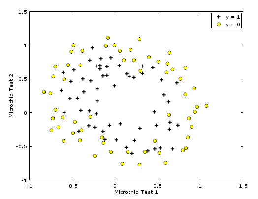{: .image-center} Figure shows that our dataset cannot be separated into positive and negative examples by a straight-line through the plot. Therefore, a straightforward application of logistic regression will not perform well on this dataset since logistic regression will only be able to find a linear decision boundary.

2.2 Feature mapping

One way to fit the data better is to create more features from each data point. In the provided function mapFeature.m, we will map the features into all polynomial terms of \(x_1\) and \(x_2\) up to the sixth power. \[ feature(x) = \begin{bmatrix} \\\ 1 \\\ x_1 \\\ x_2 \\\ x_1^2 \\\ x_1x_2 \\\ x_2^2 \\\ x1^3 \\\ . \\\ . \\\ . \\\ x_1x_2^5 \\\ x_2^6 \end{bmatrix} \]

2.3 Cost function and gradient

The regularized cost function in logistic regression is \[J(\theta) = \frac{1}{m}\sum_{i=1}^m[−y^{(i)}\log(h_\theta(x^{(i)})) − (1 − y^{(i)})\log(1 − h_\theta(x^{(i)}))] + \frac{\lambda}{2m}\sum_{j=1}^n\theta_j^2\]

The gradient of the cost function is a vector where the \(j\)th element is defined as follows:

\[ \begin{array}{lr} \frac{\partial J(\theta)}{\partial \theta_0} = \frac{1}{m}\sum_{i=1}^m\bigg(h_\theta(x^{(i)}) − y^{(i)}\bigg)x_j^{(i)} & \text{for }j = 0 \\\ \frac{\partial J(\theta)}{\partial \theta_j} = \frac{1}{m}\sum_{i=1}^m\bigg(h_\theta(x^{(i)}) − y^{(i)}\bigg)x_j^{(i)} + \frac{\lambda}{m}\theta_j & \text{for }j \geq 1 \end{array} \]

costFunctionReg.m

function [J, grad] = costFunctionReg(theta, X, y, lambda)
%COSTFUNCTIONREG Compute cost and gradient for logistic regression with regularization
%   J = COSTFUNCTIONREG(theta, X, y, lambda) computes the cost of using
%   theta as the parameter for regularized logistic regression and the
%   gradient of the cost w.r.t. to the parameters. 

% Initialize some useful values
m = length(y); % number of training examples

% You need to return the following variables correctly 
J = 0;
grad = zeros(size(theta));

% ====================== YOUR CODE HERE ======================
% Instructions: Compute the cost of a particular choice of theta.
%               You should set J to the cost.
%               Compute the partial derivatives and set grad to the partial
%               derivatives of the cost w.r.t. each parameter in theta


n = size(theta);
h = sigmoid(X*theta);

theta1 = [0 ; theta(2:n)];
p = lambda*(theta1'*theta1)/(2*m);

J=(-y'*log(h) - (1-y)'*log(1-h))/m + p;

grad = X'*(h-y)/m + lambda*theta1/m;
% =============================================================

end

2.4 Plotting the decision boundary

plotDecisionBoundary.m