1.1 Visualizing data

function plotData(X, y)
%PLOTDATA Plots the data points X and y into a new figure 
%   PLOTDATA(x,y) plots the data points with + for the positive examples
%   and o for the negative examples. X is assumed to be a Mx2 matrix.

% Create New Figure
figure; hold on;

% ====================== YOUR CODE HERE ======================
% Instructions: Plot the positive and negative examples on a
%               2D plot, using the option 'k+' for the positive
%               examples and 'ko' for the negative examples.
%


% Find Indices of Positive and Negative Examples
pos = find(y==1); neg = find(y == 0);
% Plot Examples
plot(X(pos, 1), X(pos, 2), 'k+','LineWidth', 2, 'MarkerSize', 7);
plot(X(neg, 1), X(neg, 2), 'ko', 'MarkerFaceColor', 'y', ...
    'MarkerSize', 7);

% =========================================================================

hold off;

end

1.2 Sigmoid function

Logistic regression hypothesis is defined as: \[h_\theta(x) = g(\theta^Tx)\], where function \(g\) is the sigmoid function. The sigmoid function is defined as: \[g(z) = \frac{1}{1 + e^{-z}}\]

function g = sigmoid(z)
%SIGMOID Compute sigmoid functoon
%   J = SIGMOID(z) computes the sigmoid of z.

% You need to return the following variables correctly 
g = zeros(size(z));

% ====================== YOUR CODE HERE ======================
% Instructions: Compute the sigmoid of each value of z (z can be a matrix,
%               vector or scalar).

g = 1./(1 .+ exp(-1*z) );

% =============================================================

end

1.3 Cost function and gradient

The cost function in logistic regression is \[J(\theta) = \frac{1}{m}\sum_{i=1}^m[−y^{(i)}\log(h_\theta(x^{(i)})) − (1 − y^{(i)})\log(1 − h_\theta(x^{(i)}))]\], and the gradient of the cost is a vector of the same length as \(\theta\) where the \(j\)th element (for j = 0, 1, . . . , n) is defined as follows: \[\frac{\partial J(\theta) }{\partial \theta_j } = \frac{1}{m}\sum_{i=1}^m \bigg(h_\theta(x^{(i)}) − y^{(i)}\bigg)x_j^{(i)}\]

function [J, grad] = costFunction(theta, X, y)
%COSTFUNCTION Compute cost and gradient for logistic regression
%   J = COSTFUNCTION(theta, X, y) computes the cost of using theta as the
%   parameter for logistic regression and the gradient of the cost
%   w.r.t. to the parameters.

% Initialize some useful values
m = length(y); % number of training examples

% You need to return the following variables correctly 
J = 0;
grad = zeros(size(theta));

% ====================== YOUR CODE HERE ======================
% Instructions: Compute the cost of a particular choice of theta.
%               You should set J to the cost.
%               Compute the partial derivatives and set grad to the partial
%               derivatives of the cost w.r.t. each parameter in theta
%
% Note: grad should have the same dimensions as theta
%

h = sigmoid(X*theta);
J=(-y'*log(h) - (1-y)'*log(1.-h))/m;
grad = X'*(h-y)/m;


% =============================================================

end

1.4 Learning parameters using fminunc

Octave/MATLAB’s fminunc is an optimization solver that finds the minimum of an unconstrained function. For logistic regression, you want to optimize the cost function \(J(\theta)\) with parameters \(\theta\).

%% ============= Part 3: Optimizing using fminunc  =============
%  In this exercise, you will use a built-in function (fminunc) to find the
%  optimal parameters theta.

%  Set options for fminunc
options = optimset('GradObj', 'on', 'MaxIter', 400);

%  Run fminunc to obtain the optimal theta
%  This function will return theta and the cost 
[theta, cost] = ...
    fminunc(@(t)(costFunction(t, X, y)), initial_theta, options);

1.5 Decision boundary

This final \(\theta\) value computed from fminunc will then be used to plot the decision boundary on the training data.

\(y\) value on the decision boundary satifies: \[y = h_\theta(x) = g\bigg(\theta^Tx\bigg) = 0.5 \], that is, \[\theta^Tx = 0 \]

• When training data X has two features \(x_1\), \(x_2\), \[\theta_1 + \theta_2 * x_1 + \theta_3*x_2 = 0 \], that is, \[x_2 = -\frac{\theta_1 + \theta_2 * x_1}{\theta_3} \],

• When training data X has more than 2 features, how to visualize it on 2D plot?

function plotDecisionBoundary(theta, X, y)
%PLOTDECISIONBOUNDARY Plots the data points X and y into a new figure with
%the decision boundary defined by theta
%   PLOTDECISIONBOUNDARY(theta, X,y) plots the data points with + for the 
%   positive examples and o for the negative examples. X is assumed to be 
%   a either 
%   1) Mx3 matrix, where the first column is an all-ones column for the 
%      intercept.
%   2) MxN, N>3 matrix, where the first column is all-ones

% Plot Data
plotData(X(:,2:3), y);
hold on

if size(X, 2) <= 3
    % Only need 2 points to define a line, so choose two endpoints
    plot_x = [min(X(:,2))-2,  max(X(:,2))+2];

    % Calculate the decision boundary line
    plot_y = (-1./theta(3)).*(theta(2).*plot_x + theta(1));

    % Plot, and adjust axes for better viewing
    plot(plot_x, plot_y)
    
    % Legend, specific for the exercise
    legend('Admitted', 'Not admitted', 'Decision Boundary')
    axis([30, 100, 30, 100])
else
    % Here is the grid range
    u = linspace(-1, 1.5, 50);
    v = linspace(-1, 1.5, 50);

    z = zeros(length(u), length(v));
    % Evaluate z = theta*x over the grid
    for i = 1:length(u)
        for j = 1:length(v)
            z(i,j) = mapFeature(u(i), v(j))*theta;
        end
    end
    z = z'; % important to transpose z before calling contour

    % Plot z = 0
    % Notice you need to specify the range [0, 0]
    contour(u, v, z, [0, 0], 'LineWidth', 2)
end
hold off

end

function out = mapFeature(X1, X2)
% MAPFEATURE Feature mapping function to polynomial features
%
%   MAPFEATURE(X1, X2) maps the two input features
%   to quadratic features used in the regularization exercise.
%
%   Returns a new feature array with more features, comprising of 
%   X1, X2, X1.^2, X2.^2, X1*X2, X1*X2.^2, etc..
%
%   Inputs X1, X2 must be the same size
%

degree = 6;
out = ones(size(X1(:,1)));
for i = 1:degree
    for j = 0:i
        out(:, end+1) = (X1.^(i-j)).*(X2.^j);
    end
end

end

1.6 Evaluating logistic regression

function p = predict(theta, X)
%PREDICT Predict whether the label is 0 or 1 using learned logistic 
%regression parameters theta
%   p = PREDICT(theta, X) computes the predictions for X using a 
%   threshold at 0.5 (i.e., if sigmoid(theta'*x) >= 0.5, predict 1)

m = size(X, 1); % Number of training examples

% You need to return the following variables correctly
p = zeros(m, 1);

% ====================== YOUR CODE HERE ======================
% Instructions: Complete the following code to make predictions using
%               your learned logistic regression parameters. 
%               You should set p to a vector of 0's and 1's
%

p = sigmoid(X, theta)>=0.5;

% =========================================================================

end

%  Predict probability for a student with score 45 on exam 1 
%  and score 85 on exam 2 

prob = sigmoid([1 45 85] * theta);
fprintf(['For a student with scores 45 and 85, we predict an admission ' ...
         'probability of %f\n\n'], prob);

% Compute accuracy on our training set
p = predict(theta, X);

fprintf('Train Accuracy: %f\n', mean(double(p == y)) * 100);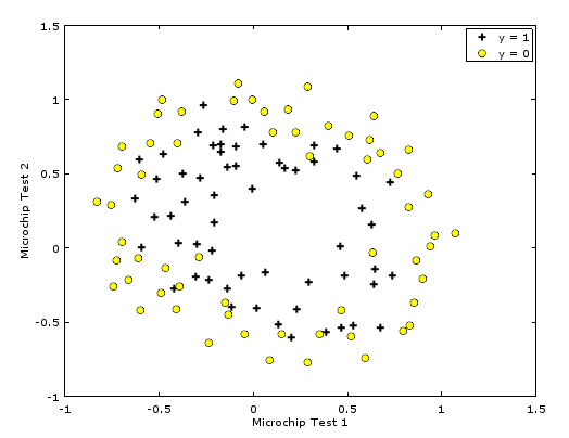

2.1 Visualizing the data

{: .image-center} Figure shows that our dataset cannot be separated into positive and negative examples by a straight-line through the plot. Therefore, a straightforward application of logistic regression will not perform well on this dataset since logistic regression will only be able to find a linear decision boundary.

2.2 Feature mapping

One way to fit the data better is to create more features from each data point. In the provided function mapFeature.m, we will map the features into all polynomial terms of \(x_1\) and \(x_2\) up to the sixth power. \[ feature(x) = \begin{bmatrix} \\\ 1 \\\ x_1 \\\ x_2 \\\ x_1^2 \\\ x_1x_2 \\\ x_2^2 \\\ x1^3 \\\ . \\\ . \\\ . \\\ x_1x_2^5 \\\ x_2^6 \end{bmatrix} \]

2.3 Cost function and gradient

The regularized cost function in logistic regression is \[J(\theta) = \frac{1}{m}\sum_{i=1}^m[−y^{(i)}\log(h_\theta(x^{(i)})) − (1 − y^{(i)})\log(1 − h_\theta(x^{(i)}))] + \frac{\lambda}{2m}\sum_{j=1}^n\theta_j^2\]

The gradient of the cost function is a vector where the \(j\)th element is defined as follows:

\[ \begin{array}{lr} \frac{\partial J(\theta)}{\partial \theta_0} = \frac{1}{m}\sum_{i=1}^m\bigg(h_\theta(x^{(i)}) − y^{(i)}\bigg)x_j^{(i)} & \text{for }j = 0 \\\ \frac{\partial J(\theta)}{\partial \theta_j} = \frac{1}{m}\sum_{i=1}^m\bigg(h_\theta(x^{(i)}) − y^{(i)}\bigg)x_j^{(i)} + \frac{\lambda}{m}\theta_j & \text{for }j \geq 1 \end{array} \]

costFunctionReg.m

function [J, grad] = costFunctionReg(theta, X, y, lambda)
%COSTFUNCTIONREG Compute cost and gradient for logistic regression with regularization
%   J = COSTFUNCTIONREG(theta, X, y, lambda) computes the cost of using
%   theta as the parameter for regularized logistic regression and the
%   gradient of the cost w.r.t. to the parameters. 

% Initialize some useful values
m = length(y); % number of training examples

% You need to return the following variables correctly 
J = 0;
grad = zeros(size(theta));

% ====================== YOUR CODE HERE ======================
% Instructions: Compute the cost of a particular choice of theta.
%               You should set J to the cost.
%               Compute the partial derivatives and set grad to the partial
%               derivatives of the cost w.r.t. each parameter in theta


n = size(theta);
h = sigmoid(X*theta);

theta1 = [0 ; theta(2:n)];
p = lambda*(theta1'*theta1)/(2*m);

J=(-y'*log(h) - (1-y)'*log(1-h))/m + p;

grad = X'*(h-y)/m + lambda*theta1/m;
% =============================================================

end

2.4 Plotting the decision boundary

plotDecisionBoundary.m

plotdata.m

function plotData(x, y)
%PLOTDATA Plots the data points x and y into a new figure 
%   PLOTDATA(x,y) plots the data points and gives the figure axes labels of
%   population and profit.

% ====================== YOUR CODE HERE ======================
% Instructions: Plot the training data into a figure using the 
%               "figure" and "plot" commands. Set the axes labels using
%               the "xlabel" and "ylabel" commands. Assume the 
%               population and revenue data have been passed in
%               as the x and y arguments of this function.
%
% Hint: You can use the 'rx' option with plot to have the markers
%       appear as red crosses. Furthermore, you can make the
%       markers larger by using plot(..., 'rx', 'MarkerSize', 10);

figure; % open a new figure window


plot(x, y, 'rx', 'MarkerSize', 10);
ylabel('Profit in $10,000s');
xlabel('Population of City in 10,000s');



% ============================================================

end

Cost function

% non-vectorized version.
J = 0;
for i=1:m
  dif = X(i, :)*theta-y(i);
  J = J + dif*dif;
endfor
J = J / (2*m);


% vectorized version.
dif = X*theta-y;
J = (dif'*dif)/(2*m);

Gradient decent

function [theta, J_history] = gradientDescent(X, y, theta, alpha, num_iters)
%GRADIENTDESCENT Performs gradient descent to learn theta
%   theta = GRADIENTDESENT(X, y, theta, alpha, num_iters) updates theta by 
%   taking num_iters gradient steps with learning rate alpha

% Initialize some useful values
m = length(y); % number of training examples
J_history = zeros(num_iters, 1);

for iter = 1:num_iters

    % ====================== YOUR CODE HERE ======================
    % Instructions: Perform a single gradient step on the parameter vector
    %               theta. 
    %
    % Hint: While debugging, it can be useful to print out the values
    %       of the cost function (computeCost) and gradient here.
    %
    
    theta_prev = theta;
    p = length(theta);

    for j = 1:p

        sum = 0;
        for i = 1:m
            sum = sum + (X(i,:)*theta_prev - y(i))*X(i,j);
        end

        derive = sum/m;
        theta(j) = theta(j) - alpha*derive;
    end


    % ============================================================

    % Save the cost J in every iteration    
    J_history(iter) = computeCost(X, y, theta);

end

end

    theta_prev = theta;
    p = length(theta);

    for j = 1:p

        derive = (X*theta_prev - y)'*X(:,j)/m;
        theta(j) -= alpha*derive;
    end

theta -= alpha*X'*(X*theta-y)/m;

Feature normalization

When features differ by orders of magnitude, first performing feature scaling can make gradient descent converge much more quickly.

• Non-vectorized version

function [X_norm, mu, sigma] = featureNormalize(X)
%FEATURENORMALIZE Normalizes the features in X 
%   FEATURENORMALIZE(X) returns a normalized version of X where
%   the mean value of each feature is 0 and the standard deviation
%   is 1. This is often a good preprocessing step to do when
%   working with learning algorithms.

% You need to set these values correctly
X_norm = X;
mu = zeros(1, size(X, 2));
sigma = zeros(1, size(X, 2));

% ====================== YOUR CODE HERE ======================
% Instructions: First, for each feature dimension, compute the mean
%               of the feature and subtract it from the dataset,
%               storing the mean value in mu. Next, compute the 
%               standard deviation of each feature and divide
%               each feature by it's standard deviation, storing
%               the standard deviation in sigma. 
%
%               Note that X is a matrix where each column is a 
%               feature and each row is an example. You need 
%               to perform the normalization separately for 
%               each feature. 
%
% Hint: You might find the 'mean' and 'std' functions useful.
%       

for p = 1:size(X, 2)
    mu(p) = mean(X(:, p), "a");
    sigma(p) = std(X(:, p));
end

for p = 1:size(X, 2)
    for i = 1:size(X, 1)
      X_norm(i, p) = (X(i, p)-mu(p))/sigma(p);
    end
end

% ============================================================

end

• Vectorized version

    mu = mean(X, "a");
    sigma = std(X);

    ones_matrix = ones(size(X));
    X_norm = (X - ones_matrix*diag(mu))./(ones_matrix*diag(sigma));

Estimate the price of a 1650 sq-ft, 3 br house, in ex1_multi.m

% ====================== YOUR CODE HERE ======================
% Recall that the first column of X is all-ones. Thus, it does
% not need to be normalized.
price = [1 ([1650 3] - mu)./sigma]*theta; % You should change this

Normal Equations

The closed-form solution to linear regression is \[\theta = (X^TX)^{-1}X^T\vec{y}\]

• Implementation

function [theta] = normalEqn(X, y)
%NORMALEQN Computes the closed-form solution to linear regression 
%   NORMALEQN(X,y) computes the closed-form solution to linear 
%   regression using the normal equations.

theta = zeros(size(X, 2), 1);

% ====================== YOUR CODE HERE ======================
% Instructions: Complete the code to compute the closed form solution
%               to linear regression and put the result in theta.
%

% ---------------------- Sample Solution ----------------------


theta = inv(X'*X)*X'*y;

% -------------------------------------------------------------


% ============================================================

end

Estimate the price of a 1650 sq-ft, 3 br house

price = [1 1650 3]*theta; % You should change this

2.1. Create my own sublime-build for R markdown files

The default build system of R-box doesn’t work, and get the error

Error: '\G' is an unrecognized escape in character string starting "'C:\G"
Execution halted
[Finished in 0.4s with exit code 1]

since the windows path escape is not correctly handled.

This issue can be resolved by regular expression replacement ¹

{
    "selector": "text.html.markdown.rmarkdown",
    "working_dir": "${project_path:${folder}}",
    "cmd": [
        "Rscript", "-e",
        "library(rmarkdown); render('${file/\\\\/\\/\/g}')"
    ]
}

2.2. Apply fix for pandoc 1.4 ²

To support latex in R markdown document, I added to the file …3.tex:

    %fix for pandoc 1.14
    \providecommand{\tightlist}{
      \setlength{\itemsep}{0pt}\setlength{\parskip}{0pt}}